Developability screening
Rank candidates on how strongly they associate with themselves.
Self-interaction data sits next to SEC and DLS in an early panel.
self-interaction

Label-free interaction analysis measures real-time binding of molecules. It adds a functional readout next to size and particle methods, covering how much protein still binds and how strongly a molecule associates with itself.
Rank candidates on how strongly they associate with themselves.
Self-interaction data sits next to SEC and DLS in an early panel.
Find the conditions that keep protein binding-competent.
Compare binding activity across buffers, alongside nanoDSF thermal data.
Measure what still binds after applied stress.
Stress the material offline, then read activity at controlled analysis temperature.
Characterise the antibody response to a biotherapeutic.
Kinetic ADA characterisation next to a bridging ELISA titer.
Follow elongation on immobilised seeds in real time.
Binding kinetics next to ThT fluorescence and electron microscopy.
Discuss your assay with one of our application specialists.

Four addressable flow channels, four sensors each, with the sample passing through them in series.
Self-association shows up as binding response, which ranks candidates on aggregation propensity before formulation work begins.
Amyloid-beta seeds are held on the sensor and monomer is injected over them, with the response recorded through the whole injection.
The inQuiQ768 autosampler takes 2×96 or 2×384 well plates and injects one sample after another, so every candidate meets the same surface.
Every sample follows the same five steps. A conformation-selective antibody is held on the sensor, the sample flows past, and the response is recorded through the whole injection. Assembled material binds; monomer does not.
A conformation-selective capture antibody is coupled to the sensor surface.
It recognises an epitope that only exists once subunits assemble. For amyloid-β that means oligomer and protofibril are captured while monomer is not.
Unused activated sites are switched off before the first sample arrives.
Excipients, surfactant and carrier protein reach the surface with every injection. Deactivation, together with the antifouling hydrogel, keeps them out of the sensorgram.
The sample is injected. Aggregate binds, monomer flows straight past.
Each aggregate is caught across several arms at once, so the surface loads quickly. The plateau reads assembled content rather than total protein.
Buffer replaces the sample and the response barely moves.
A multivalent complex has a very slow koff, so the captured material stays bound and only a small fraction releases. The signal that holds is what gets read across a stress timepoint series.
A regeneration buffer returns the sensor to baseline for the next sample.
Buffer alone will not clear an avidity-locked complex, so the surface is stripped deliberately. Every timepoint and every formulation then meets the same antibody layer.
Six capabilities, one modular benchtop instrument, in a label-free workflow.
Immobilise the candidate and inject the same molecule. Weak self-association shows up as binding response, which ranks candidates on aggregation propensity.
A standard curve of the reference material turns binding response into the concentration of protein that still engages its target.
The antifouling hydrogel limits binding by matrix and excipient components, with samples clarified through 0.22 µm before injection.
SEC, AUC, mass photometry, and light obscuration report how much aggregate is present. Binding data reports whether the rest still works.
kon, koff, and KD are measured the same way in developability, formulation, and stability studies, so the numbers compare across the workflow.
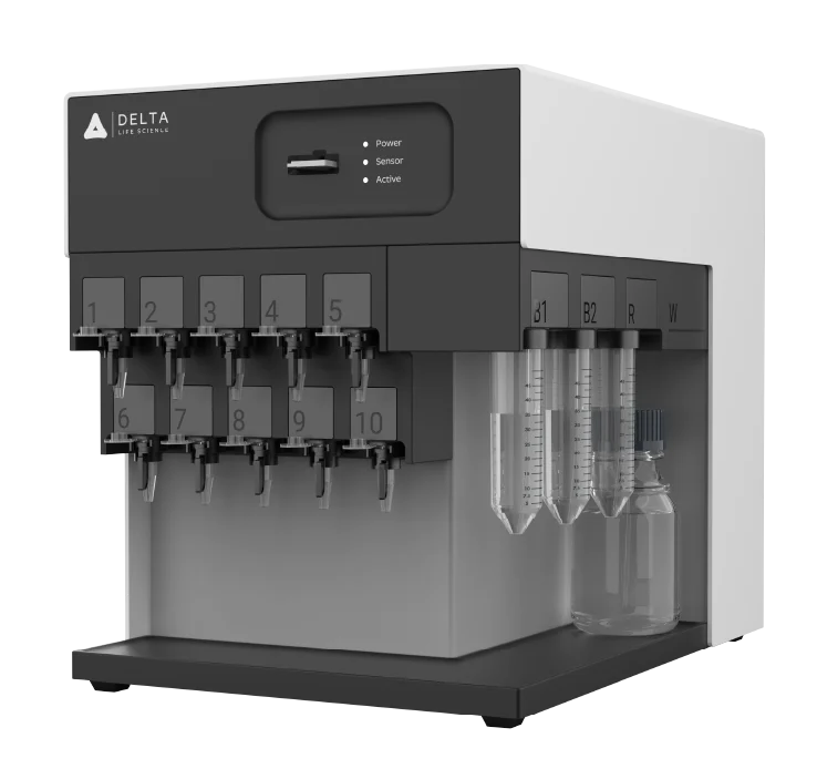
The autosampler takes 2×96 or 2×384 well plates and works through candidate panels one injection after another.
Label-free binding analysis does not size or count aggregates. SEC, DLS, AUC, and light obscuration do that. What a binding measurement adds is the other half of the question, namely how much of the material still engages its target and how strongly the molecule associates with itself. The two run alongside each other rather than one replacing the other.
Rank candidates on self-interaction and on retained target binding. A molecule that associates strongly with itself carries a higher aggregation and viscosity risk later in development, and a candidate that loses target binding under a formulation condition is telling you something a size profile will not.
Immobilise the molecule on the sensor and inject the same molecule as a concentration series. The response reflects how readily the protein binds to itself, which ranks candidates on aggregation propensity under a defined buffer condition.
It reports a change in binding behaviour rather than the presence of aggregate. Biphasic dissociation, poor fits to a 1:1 model, and a drifting maximum response all have several possible causes, including mass transport, surface heterogeneity, and ligand inactivation. Assign the cause with an orthogonal size method, then use the binding data to say whether the remaining material still works.
Apply the stress offline, then inject the stressed material and the unstressed reference against the same capture surface. The instrument controls the analysis temperature, so the comparison is made under one set of conditions and differences in active concentration or in kon and koff can be attributed to the applied stress.
Capture the therapeutic on the sensor and inject patient or animal serum. The response gives a kinetic profile of the anti-drug antibody response, with kon, koff, and KD alongside the titer a bridging ELISA reports.