Domain-level interactions
Find out which part of a multi-domain protein carries the binding.
Compare truncations and mutants against the full-length protein.
competitive assays

Label-free interaction analysis measures binding between unmodified molecules in real time. For structural biology, it returns affinity, association and dissociation rates, and specificity in solution.
Find out which part of a multi-domain protein carries the binding.
Compare truncations and mutants against the full-length protein.
Test an AlphaFold or docking prediction at the bench.
Measure KD to test the predicted interface.
Confirm a construct still binds the way its parent does.
Compare stabilised, truncated, and mutated variants side by side.
Check that the complex forms before structural work.
Confirm binding and complex stability before committing beam or microscope time.
Measure the same interaction across temperatures.
Add a temperature series to the binding measurement.
Discuss your assay with one of our application specialists.

Four independently addressable flow channels, each carrying four sensors, with the sample flowing through the channels in series.
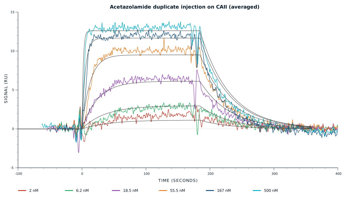
The association phase gives kon, the dissociation phase gives koff, and together they give KD. Affinity runs from 10 pM to 10 mM, with steady-state fitting where dissociation is too fast for kinetics.
The analytes stay unmodified in solution, so it measures native interactions without label or tag artifacts.
Compare full-length protein with truncations and point mutants to identify the construct that retains affinity and localise the interaction.
Every measurement follows the same steps, whatever the complex. One partner is immobilised on the sensor, the other flows past, and the instrument records the response in real time. An endpoint assay gives you one number. The inQuiQ gives you the full curve.
One binding partner is attached to the sensor surface first.
Amine coupling or tag capture immobilises the protein. The more stable or readily produced partner is usually immobilised, while the other is injected. Ligand density is optimised to avoid mass-transport limitation.
Any activated site left unused is deactivated before the first sample arrives.
Without it the surface keeps reacting with sample passing over, and non-specific binding shows up in the trace as signal that has nothing to do with the pair being measured. The response settles at a stable level, the immobilised amount.
The second partner flows across the surface and the response climbs.
During association, the injected analyte binds to the immobilised target, and the rising response reflects how quickly the complex forms. The association phase determines the on-rate, kon.
Buffer replaces the sample and the response falls as the complex comes apart.
The dissociation phase gives the off-rate, koff; 1/koff gives complex lifetime. A concentration series gives kon, koff, and KD across 10 pM to 10 mM. For fast dissociation, plateau responses give steady-state affinity. Single-cycle kinetics runs the series uninterrupted when protein is scarce.
A regeneration buffer strips the bound partner and returns the sensor to baseline, ready for the next injection.
The immobilised partner stays in place, so every variant meets the same surface. Inject, read, regenerate, repeat, unattended. Each injection is read by every sensor, so one sample can cover multiple constructs, mutants, or controls.
Six capabilities, one modular benchtop instrument, in a label-free workflow.
4-plex with in-flow immobilisation and 16-plex with a spotter lets you compare truncations, point mutants, and controls from one sample.
Baseline noise stays low enough that a small binding response is still readable.
One affinity range covers weak contacts through tight complexes, with steady-state fitting when kinetics are too fast.
Competitive and blocking assays identify the construct or domain carrying the binding.
The temperature-controlled flow cell runs a full temperature series.
Simply add an autosampler, and run a long variant or condition series unattended.
Cryo-EM, X-ray crystallography, and NMR give structure. Label-free interaction analysis, ITC, mass photometry, and SEC-MALS give function and behaviour in solution. Label-free analysis with the inQuiQ adds affinity (KD) and kinetics (kon, koff), so you can show that a modelled interface produces measurable, specific binding under native conditions.
Express the predicted partners, measure their binding in solution, and compare the result with the prediction. A measured KD and a clean sensorgram support the model. Competitive assays against truncations or point mutants then test whether the predicted interface is the one that actually drives binding.
The inQuiQ runs from 30 µL of sample. Sensors are regenerable, so the same chip carries a series of variants, mutants, and controls rather than one measurement per surface. That matters for structural constructs that are slow to express or purify.
Yes, indirectly and reliably. Run the full-length protein on the inQuiQ and its truncations or domain constructs as separate binding experiments, then use competitive and blocking assays to see which construct carries the affinity. The comparison localises the interaction without needing a new structure for every variant.
Affinity (KD) says how tightly two molecules bind at equilibrium. Kinetics says how they get there: kon for how fast the complex forms, koff for how fast it falls apart. Two complexes can share a KD and behave differently, which is why structural work benefits from both.